DSP: Python Implementation of Persistent Spectrum Analysis
September 2025 (2282 Words, 13 Minutes)
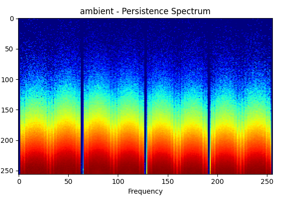 A Persistence Spectrum Visualization of background RF noise
Radio frequency signal analysis in Python should be straightforward, but it’s not. While Python is great at machine learning, it lacks the signal analysis tools that MATLAB provides out-of-the-box functions for, with the most obvious missing piece: the persistent spectrum.
Standard Python libraries offer basic PSD (scipy.signal.welch) and spectrogram (scipy.signal.spectrogram) functions, but they’re missing a huge capability: persistent spectrum analysis. This visualization technique reveals weak, intermittent signals that traditional methods completely miss and is absolutely crucial for signal analysis.
This tutorial fills that gap by implementing persistent spectrum analysis in Python and bringing this to the ML/Python community.
The Problem: Hidden Signals in RF Data
When analyzing RF signals, we often need to detect weaker signals that appear sporadically against stronger background signals. The traditional spectral analysis visualizations struggle with this because:
Power Spectral Density (PSD) averages power across the entire recording duration. When a weak signal appears only for a short time, it gets diluted by all the time periods where it’s absent. This results in the weaker signal not showing up at all.
Spectrograms show the time-frequency content but display signals at similar intensity whether they appear constantly or just occasionally. Weaker, non constant signals become easy to overlook against background noise. The weaker signals show up but are often small and are missed at a glance.
What we need is a way to see not just when frequencies occur, but how consistently they occur at different power levels.
This is exactly why we need a persistent spectrum and unfortunately, Python’s standard libraries do not include this functionality.
Persistent Spectrum in Python
To show why persistent spectrum is such an important feature, I’ll use a test signal from this MATLAB document that combines:
- A chirp signal (frequency sweep from 180-220 Hz) with noise; a stronger signal that is very visible
- A weak 210 Hz tone that appears only in the first 1/6 of the recording; a weaker signal that is embedded inside of the stronger one
This is a classic problem in signal detection where we attempt to identify a sparser signal against the background of stronger signal and noise.
import matplotlib.pyplot as plt
import numpy as np
from scipy.signal import chirp

fs = 1000
t = np.arange(0, 500, 1/fs)
x = chirp(t, 180, t[-1], 220) + 0.15 * np.random.randn(len(t))
idx = int(np.floor(len(x)/6))
x[:idx] = x[:idx] + 0.05*np.cos(2*np.pi*t[:idx]*210)
Below is the implementation of what the example signal looks like plotted like a spectrogram and a persistence spectrum in MATLAB.
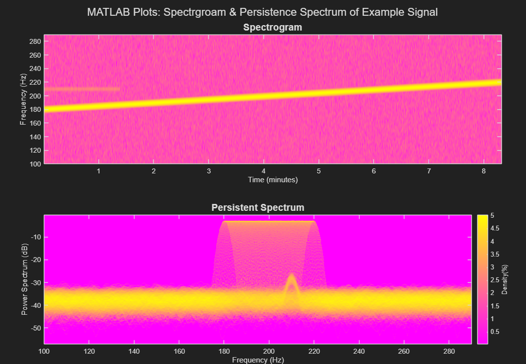
As we can see, the smaller signal is embedded inside the larger signal. Note how the weak signal is barely visible in the spectrogram but clearly revealed in the persistent spectrum.
For situations like these, using a spectrogram alone would not be sufficient and would miss the weaker signal entirely.
Python Stock Functions for Signal Analysis
Python offers several built in functions in common packages for signal processing which I will go over here.
PSD Implementations
For plotting a PSD in Matplotlib, there is a built in function matplotlib.pyplot.psd() that can be used as follows:
plt.psd(x, Fs=fs)
The function scipy.signal.welch() is the most commonly used PSD function in Python:
f, psd = welch(x, fs, nperseg=1024, noverlap=None)
Result: The weaker signal is completely invisible! The PSD does not show the weaker signal at all. This is what we expect and why we cannot use the PSD alone.
Spectrogram Implementations
Matplotlib also provides plt.specgram():
plt.specgram(x, NFFT=256, Fs=fs, noverlap=128, cmap='PiYG')
This SciPy’s implementation of a spectrogram with the default parameters:
f, t, Sxx = spectrogram(x, fs, nperseg=1024)
Result: While we can see the signal, the signal is barely visible. This makes it easy to overlook against the background noise.
The limitation is clear: we need to see not just when frequencies occur, but how consistently they occur.
Implementing Persistent Spectrum in Python
To bridge this gap, I’ll adapt the implementation approach from this original blog post that successfully recreated MATLAB’s persistent spectrum functionality. While the core algorithms remain the same, I’ll walk through how to implement them in Python and explain why they work.
Credit goes to Xiao Lio and his blog for the initial implementation! My contribution is making these techniques accessible to the Python/ML community with clear explanations and working code.
The implementation consists of three main parts:
-
Helper functions for efficient windowing and spectral analysis
-
Core spectral processing with optimized parameters
-
Persistent spectrum generation that reveals intermittent signals
Helper Functions
First, let’s implement the two core helper functions that make efficient spectral analysis possible:
Windowing Function
This function creates overlapping views of our signal without copying the data. Allows for processing of long RF recordings without running out of memory.
def _stride_windows(x, n, noverlap=0):
    """
    Create overlapping windows using NumPy stride tricks for memory efficiency.
    Adapted from matplotlib's implementation but simplified.
    """
    noverlap = int(noverlap)
    n = int(n)
    step = n - noverlap
    shape = (n, (x.shape[-1]-noverlap)//step)
    strides = (x.strides[0], step*x.strides[0])
    return np.lib.stride_tricks.as_strided(x, shape=shape, strides=strides)
STFT calculation
This is the main STFT function that is used to calculate both the spectrogram and persistence spectrum:
- Multiplying each data segment by set the Kaiser window
- Apply the STFT to each segment and then convert it to power
- For signals comprised of complex numbers: shifts the result so that the DC at 0 is in the middle of the graph
- For signals comprised of real numbers: it discards the negative frequency comp
The key improvement here are:
- Kaiser windowing (β=20) instead of default Hanning for better spectral leakage control
- Proper normalization ensuring correct dB/Hz scaling
- Efficient memory usage through stride tricks
def _spectral_helper(x, Fs=1, NFFT=1024, noverlap=0):
    """
    Core spectral analysis with proper windowing and normalization.
    """
    # Use Kaiser window
    window = np.kaiser(NFFT, 20)

    # Create windows
    result = _stride_windows(x, NFFT, noverlap)
    result = result * window.reshape((-1, 1))

    # Apply FFT and convert to power
    result = np.fft.fft(result, n=NFFT, axis=0)
    result = np.real(np.conj(result) * result)
    freqs = np.fft.fftfreq(NFFT, 1/Fs)

    if not np.iscomplex(x[0]):
        result = result[:NFFT//2 + 1, :]
        result[1:, :] *= 2
        freqs = freqs[:NFFT//2 + 1]
        freqs[-1] *= -1

    # Proper normalization in dB/Hz units
    result /= Fs
    result /= (np.abs(window)**2).sum()

    t = np.arange(NFFT/2, len(x) - NFFT/2 + 1, NFFT - noverlap)/Fs
    return result, freqs, t
2. Main Functions
Main Analysis Functions
Now, with those helper functions, we can take the STFT and convert it to our visualizations:
Custom Spectrogram
The persistent spectrum creates a histogram of power levels for each frequency. Instead of showing power over time, it shows how often each power level occurs:
def generate_stft(x, fs, nfft, noverlap, plot=True):
    """
    Optimized spectrogram using MATLAB implementation
    """
    result, freqs, t = _spectral_helper(x, Fs=fs, NFFT=nfft, noverlap=noverlap)
    stft = 10 * np.log10(result + 1e-6)

    if plot:
        pad_xextent = (nfft - noverlap) / fs / 2
        xmin, xmax = np.min(t) - pad_xextent, np.max(t) + pad_xextent
        extent = xmin, xmax, freqs[0], freqs[-1]

        plt.figure(figsize=(12, 8))
        plt.imshow(stft, cmap="spring", extent=extent,
                  vmin=-50, vmax=0, origin='lower')
        plt.ylim([100, 290])
        plt.ylabel('Frequency (Hz)')
        plt.xlabel('Time (s)')
        plt.title('Spectrogram')
        plt.colorbar(label='Power (dB)')
        plt.show()

    return stft
Persistence Spectrum
We can think of the Persistence Spectrum as a sort of Histogram on the results of the SFTF. So, Xiao’s implementation basically plots the result of the SFTF as a histogram:
def generate_pspectrum(x, fs, nfft, noverlap, nbins, plot=True):
    """
    Generate persistent spectrum using MATLAB implementation
    """
    result, freqs, t = _spectral_helper(x, Fs=fs, NFFT=nfft, noverlap=noverlap)
    stft = 10 * np.log10(result + 1e-6)

    # Create the persistence spectrum
    pspectrum = np.zeros((nbins, len(freqs)))
    pwr_min, pwr_max = -50, 0

    # For each frequency, create histogram of power levels over time
    for idx_f in range(len(freqs)):
        pspectrum[:, idx_f], _ = np.histogram(
            stft[idx_f, :],
            bins=np.linspace(pwr_min, pwr_max, nbins+1),
            density=False
        )

    # Apply log scaling to enhance visibility
    pspectrum = np.log(pspectrum + 0.5)

    if plot:
        plt.figure(figsize=(12.5, 6))
        plt.imshow(pspectrum, aspect="auto", cmap="spring",
                  extent=(freqs[0], freqs[-1], pwr_min, pwr_max),
                  origin='lower')
        plt.xlim([100, 290])
        plt.xlabel('Frequency (Hz)')
        plt.ylabel('Power Spectrum (dB)')
        plt.title('Persistent Spectrum')
        plt.colorbar(label='Density (log scale)')
        plt.show()

    return pspectrum
Finale
The Results: The Magic of a Persistent Spectrum
Now let’s see our custom implementation reveal the hidden signal:
stft = generate_stft(x, fs=1000, nfft=1024, noverlap=782, plot=True)
pspectrum = generate_pspectrum(x, fs=1000, nfft=1024, noverlap=782, nbins=256)
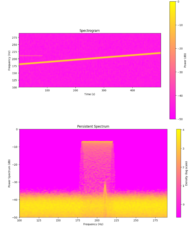
The need is clear:
With the Custom Spectrogram, Both signals are visible, but the weak 210 Hz tone appears as a faint horizontal line.
However with the Persistent Spectru, the weak signal now appears as a bright vertical feature at 210 Hz. This is very hard to miss!
This allows us to not only when frequencies occur but also now how often.
Conclusion
By implementing persistent spectrum analysis in Python, we’ve solved a limitation in the open-source signal processing space. While Python excels at machine learning, there was no easy way to use this visualization technique that’s essential for detecting weak, intermittent RF signals.
This implementation allows Python users to tackle advanced signal detection without relying on MATLAB and apply advanced ML techniques in the signal processing domain.